A trick for plotting sums of absolute value functions.

Once you know a what's going on with absolute values, you can find some shortcuts for plotting them. Of course, we don't get license to take shortcuts until we've taken a few "longcuts". (You know how we are about that.)

As an example, suppose we want to plot the graph of y=f(x), where

f(x) = |x+2| - 2x.

It is plotted below. But we need to be able to understand why it looks this way. Why the bend where x=-2, for instance? (Notice that we are not using a "true" scale for our horizontal and vertical.)

In[59]:=

Out[59]=

Think about the definition of absolute value:

|t| = {

This means that we have

|x+2| = {

and this simplifies to

|x+2| = {

Now we'll add the term 2x into the mix. (We note that 2x doesn't care if x≥2 or not!) So  

|x+2| - 2x  = {

Simplifying gives

|x+2| - 2x  = {

This means that our function f(x) = |x+2|-2x  is identical to the piecewise-linear function

f(x)  = {

Below we'll plot the line y = -x+2 in green, and the line y = -3x-2 in red.

In[71]:=

Out[71]=

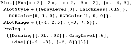
If we now throw in our absolute value function, you can see what's happening. Look below and notice the "split" at x=-2, just as we have in the piecewise-defined version of the function above. We only get the "green" part, the line y=-x+2, when x≥-2. When x<-2 we get the "red" part, the line y=-3x-2.

In[77]:=

Out[77]=

Here's a better version, including a "true" aspect ratio (equal horizontal and vertical scaling).

In[79]:=

Out[79]=

If you think about what just happened, you can see that when adding absolute values of linear functions to other linear functions, we'll always get a piecewise-linear function. Also, we'll get a "split" or "vertex" wherever the function inside the absolute value is zero. Knowing this in advance, we can "cheat"...

In the example above, we see that our vertex occurs where x+2=0, or where x=-2. Recalling that our function is f(x) = |x+2| - 2x, we see that the y-value at x=-2 will be f(-2) = -4. So the point (-2,-4) will be on our graph.

To the right of this point (i.e., where x>-2) we get a straight line, so we pick any value of x>-2, an easy one being  x=0. Since f(0)=2, we have the point (0,2).

Looking left of x=-2 (i.e., where x<-2), we can take x=-3, say. We get f(-3) =|-3+2|-2(-3)=1+6=7, so (-3,7) is on our graph.

Plotting these three points,  (-2,4), (0,2), (-3,7), on a graph and "connecting the dots" we get our picture.

In[74]:=

Out[74]=

Created by Mathematica  (June 17, 2006)